Diffraction and the Airy Disk: Optical Resolution and Point Spread Function
The Airy disk is the central bright spot formed when a perfect lens images a point source through a circular aperture. It is not an imperfection, and it is not caused by bad focusing. It appears even in a mathematically perfect optical system because light behaves as a wave.
That is why diffraction is the real lower bound on sharpness. Even if aberrations are fully corrected and sensor pixels are infinitely small, a point in the scene cannot map to a true point on the image plane. It maps to a finite spot with rings. In imaging language, this spot is the system’s point spread function (PSF).
If you work in graphics, this is immediately familiar. The PSF is a physically grounded blur kernel. Convolution with that kernel is what converts ideal scene radiance into a finite-resolution image. The same concept sits behind anti-aliasing filters, sensor MTF curves, and practical lens behavior.
Diffraction at an Aperture: Why a Point Becomes a Pattern
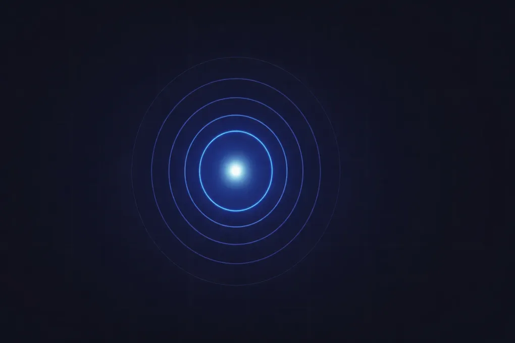
A circular aperture does not pass a point wavefront unchanged. Each point across the pupil contributes a secondary wavelet, and those wavelets interfere in the focal plane. For a circular pupil, the resulting intensity pattern is rotationally symmetric: a bright core with weaker concentric rings. That pattern is the Airy pattern, and the bright core is what people call the Airy disk.
A useful formula is the first-minimum radius in the image plane:
Where:
- is wavelength
- is focal length
- is aperture diameter
The ratio is the f-number , so the same formula is often written as . This explains the key practical tradeoff: closing the aperture (higher f-number) increases depth of field but also increases diffraction blur size.
| first dark ring radius r1 = 9.5 um | f/14.2
When you move the aperture slider, focus on the orange first-ring marker and the radial intensity profile. A larger aperture concentrates more energy in a smaller central lobe, which means better diffraction-limited detail. Changing wavelength also matters. Longer wavelengths produce a wider Airy core, which is one reason blue light can support slightly finer diffraction-limited resolution than red light under equal optics.
Angular Resolution and the Rayleigh Criterion
The Airy disk turns into a resolution rule when two nearby point sources overlap. In astronomy this might be two stars. In microscopy it might be two fluorophores. In machine vision it might be two tiny highlights on metal edges.
A standard criterion is Rayleigh’s criterion:
This is angular resolution in object space. Two equally bright points are “just resolved” when the main maximum of one Airy pattern lands at the first minimum of the other. At this spacing, you still see two peaks, but the dip between them is shallow.
| thetaR = 1.73 arcsec | sep/thetaR = 1.00 | valley dip = 26%
Try three settings for intuition by changing aperture and wavelength while keeping separation fixed, then by changing separation:
Separationlower than the currentthetaR: profiles merge into one broad bump.Separationclose to the currentthetaR: two maxima appear with the classic Rayleigh dip.Separationwell above the currentthetaR: peaks separate clearly and the dip gets deeper.
This is important because “resolution” is not a single yes/no wall. What you can detect also depends on contrast, detector noise, and post-processing. Rayleigh gives a robust physical baseline, not the final word for every task.
Airy Disk as the Point Spread Function (PSF)
In linear shift-invariant imaging, the captured image is the object irradiance convolved with the PSF:
If the system is diffraction-limited and aberrations are negligible, the PSF is the Airy pattern. This gives a direct bridge from wave optics to rendering and image processing.
For rendered lens models, this is the physically motivated blur kernel for ideal circular pupils. For real cameras, you combine this with aberration, sensor sampling, demosaic behavior, and motion blur. But diffraction is still the base floor that does not disappear.
| cutoff fc = 227 cycles/mm | freq/fc = 0.53 | contrast transfer = 62%
The third visualization shows exactly this convolution idea on repeated detail. As frequency approaches optical cutoff, contrast transfer falls even if the pattern is still nominally present. That is why images can look “soft” before features fully vanish. This is also why MTF charts matter more than only quoting megapixels.
Cutoff Frequency and MTF Intuition
For incoherent imaging with a diffraction-limited circular aperture, a common cutoff estimate is:
Here is spatial cutoff frequency on the sensor plane. Above this frequency, ideal diffraction transfer is zero. Below it, contrast decreases continuously with frequency.
This matters in practical lens selection:
- A lens at a very high f-number can become diffraction-limited before sensor sampling is the bottleneck.
- A lens at a very low f-number may be aberration-limited instead, so stopping down can improve real sharpness first, then eventually lose sharpness to diffraction.
- The best aperture for detail is often a middle value where aberration blur and diffraction blur are jointly minimized.
If this tradeoff feels similar to filter design in graphics, that is because it is. You are balancing passband behavior, cutoff behavior, and sampling constraints under a physically fixed kernel family.
Why This Topic Is Often Underexplained
A common explanation online is “smaller aperture makes everything less sharp because diffraction,” then it stops there. That misses the deeper model readers need:
- Diffraction gives the PSF shape.
- The PSF defines convolution blur.
- Convolution blur defines MTF and contrast transfer.
- Contrast transfer controls whether fine structure is still useful for downstream perception or algorithms.
Without this chain, readers memorize isolated formulas but cannot reason about real imaging systems. Once you keep the chain intact, design decisions become clearer: choosing aperture, deciding pixel pitch, interpreting lens tests, or designing physically plausible camera effects in rendering.
Practical Workflow for Real Systems
When evaluating resolution limits in a camera, microscope, telescope, or render pipeline, use this order:
- Compute the diffraction scale from and aperture (
r1in sensor units orthetaRin angular units). - Compare that scale to sensor sampling pitch and reconstruction method.
- Check whether current settings are likely aberration-limited or diffraction-limited.
- Evaluate contrast transfer at task-relevant frequencies, not just “can I barely resolve two points?”
- Validate with representative scene detail, not only synthetic line pairs.
That workflow keeps wave optics, imaging engineering, and rendering intuition in one consistent framework. If you want related intuition building blocks, the article on light refraction and Snell’s law and the breakdown of vertex and fragment shaders in the graphics pipeline provide useful complements for how light transport and sampling stages combine in real image formation.
Recap
The Airy disk is the smallest spot a perfect circular optical system can form, and it exists because of diffraction, not optical defects. From there, everything follows naturally:
- Airy pattern is the diffraction-limited PSF.
- PSF convolution sets blur and contrast behavior.
- Rayleigh gives a practical baseline for point separation.
- MTF/cutoff explain why detail fades before disappearing.
Once these pieces are connected, diffraction stops being an isolated formula and becomes a working model you can use in optics, imaging, and rendering.